9 minutes
LLM Fine-Tuning Optimization Part 2: Achieving Stability
Originally published on Substack, Nov 4, 2025
In the LLM Fine-Tuning and the Performance Tug-of-War post, we explored the constant balancing act between quality, speed, and memory when fine-tuning large language models that align with your goals and constraints. Fine-tuning is the process of teaching an existing model (e.g. GPT-NeoX, Llama, Gemma, etc.) new knowledge or behaviors, transforming a general-purpose LLM into one that is a domain specialist.
The previous post introduced the core levers of sequence length, optimizers, attention type, and LoRA, which define how a model learns, generalizes, and scales. This post expands on your optimization toolkit by introducing four more essential levers: batch size, mixed precision, quantization, and gradient checkpointing.
These aren’t nice-to-have optimizations. They determine whether your model fits in VRAM, how efficiently your GPU runs, and whether you can afford to fine-tune at all.

Frameworks and PyTorch
When you fine-tune an LLM, you typically use a framework that abstracts away low-level PyTorch details. Axolotl, Hugging Face TRL, and LLaMA-Factory let you define your entire fine-tuning setup in a YAML or JSON config file. They handle everything under the hood: loading models, setting up optimizers, managing distributed training, and implementing the optimization techniques we’re covering in these posts.
These frameworks wrap around PyTorch, the de facto standard for deep learning, handling the complex GPU calculations (tensors) and automatic gradient tracking needed to actually train and fine-tune a model. PyTorch dominates because of its flexibility, extensive ecosystem of pre-trained models, and strong support for the distributed training needed for large models. While alternatives like JAX/Flax exist, the vast majority of training and fine-tuning happens in the PyTorch ecosystem.
This matters because many of the parameters we’ve covered like Flash-style attention, LoRA, AdamW variants are surfaced by your framework as config features. When you set gradient_checkpointing: true or quantization: “8bit” in YAML, you’re telling the framework to enable specific PyTorch optimizations.
Framework-specific implementation notes: While most parameters work consistently across frameworks, implementation details can vary because they map to different backends. For example:
- Gradient checkpointing works across Axolotl, TRL, and LLaMA-Factory, but the exact checkpoint pattern may differ.
- Flash/SDPA Attention have it so some frameworks bundle a fused backend; others require manual installs or a flag to use PyTorch SDPA.
- LoRA: default ranks and target modules differ (e.g., q_proj, v_proj, o_proj).
Always check your framework’s documentation for parameter-specific behavior when switching.
🧩 More Core Config Levers / Parameters
5. Mixed Precision: The Foundation
A neural network is a giant collection of numbers, or weights, that represent its “knowledge.” By default, computers store each of these numbers in a 32-bit format (called fp32) to be highly accurate. The problem is, this format is too slow and VRAM-intensive for massive LLMs.
Mixed Precision Training is the industry-standard that uses a smaller, 16-bit format for the vast majority of calculations, cutting VRAM usage in half and unlocking your GPU’s Tensor Cores which are specialized hardware built for accelerated 16-bit math. It’s called “mixed” because it strategically keeps a few critical calculations in full 32-bit format to maintain numerical stability.
Picture it like this: fp32 is a high-resolution photo with full color depth. A 16-bit format is a slightly compressed version that looks nearly identical but is half the file size which is the perfect balance of quality and efficiency.
Formats:
- bf16 (bfloat16): modern default on A100/H100; wide dynamic range like fp32, slightly less precision; very stable.
- fp16: older; higher precision within a smaller range; may need loss scaling and can lead to very low precision.
Usage Example:
yaml

bf16: true
# Fallback for GPUs without bf16 support:
# fp16: true
Recommendation: Use bf16 if your GPU supports it (A100/H100 and some newer consumer SKUs). Otherwise use fp16. Mixed precision is non-negotiable for LLM fine-tuning.
6. Batch Size: The Throughput Lever
Batch size (how much data the model processes at once) directly affects GPU efficiency, VRAM usage, and model stability. Larger batches improve throughput by saturating your GPU, but they can exhaust VRAM quickly. Smaller batches fit easily but can lead to unstable training. If you can’t fit a large batch, use micro‑batches + gradient accumulation to simulate one for lower VRAM cost. Normally, the model updates its weights (its “knowledge”) after every single batch but gradient accumulation groups batches into updates.
It’s like building one sharp photo from eight blurry shots. You average the noise to get a cleaner image (stable gradients). Micro-batches let you process each shot without blowing VRAM, then accumulate and update once as if it were a single large batch
To help define the effective batch:
effective_batch = micro_batch_size × gradient_accumulation_steps × num_devices.
Usage Example:
yaml

micro_batch_size: 1
gradient_accumulation_steps: 8
This simulates an effective batch size of 8 (1 x 8) while keeping the per-step VRAM cost minimal.
Recommendation: Start small (micro-batch = 1) and scale up through accumulation once stability is confirmed. This approach prevents OOM errors while you’re still calibrating your setup.
7. Gradient Checkpointing: The Memory Lifeline
During fine-tuning, a model does a forward pass (making a prediction with data) and a backward pass (learning from its mistake and updating weights). To learn, the backward pass needs to look at the calculations, or activations, from the forward pass.
Gradient checkpointing saves only selected activations instead of storing all of them and recomputes the rest on the backward pass, which can free ~30-60% VRAM for only a ~10-40% speed hit.
- Standard fine-tuning (no checkpointing)
It’s like editing a photo with 100 filters and your app saves a full preview after every filter in the history. When you want to undo/redo (backward pass), it’s instant because every intermediate preview is cached—but your RAM fills up fast. - Gradient checkpointing
Same 100 filters, but your app only saves a few key previews (say after filter 1, 50, and 100). If you undo to step 75, the app replays filters 51→75 to rebuild that preview. That costs extra time, but your RAM usage stays much lower.
Gradient checkpointing is so essential that it often determines whether your configuration runs at all. It’s the lifeline you pull when your other core levers (long sequence length, large batch, or no quantization) don’t fit in VRAM.
Enable it once, benefit forever:
yaml

gradient_checkpointing: true
Recommendation: Enable gradient checkpointing by default unless you have abundant VRAM and speed is critical. The slowdown is usually a bargain for VRAM savings.
8. Quantization: Precision vs. Efficiency
Quantization is one of the most powerful techniques for making large model fine-tuning feasible on limited hardware. At its core, it’s a simple trade-off: use less precise numbers to represent model weights, and in return, use dramatically less VRAM. Quantization is a much bigger area to cover but for now, we’ll cover highlights in regards to fine-tuning.
How It Works: Quantization reduces model weights from 16-bit or 32-bit floats to lower-bit formats (8-bit or 4-bit). A 16-bit weight stores numbers with high precision (like a RAW photo), while an 8-bit weight uses less detail (like a JPEG). The model still works, but with less numerical precision per weight. This can cut VRAM by up to 75% and speed up both training and inference which makes it essential for large models on limited GPUs. However, aggressive quantization can degrade reasoning and coherence.
QLoRA Connection: Quantization is most commonly used with LoRA (covered in the previous post) in a technique called QLoRA. This combines low-precision base model weights with full-precision LoRA adapters, letting you fine-tune massive models on consumer hardware. When you see “4-bit LoRA” in the wild, that’s QLoRA.
Hardware Reality: If you’re running a 13B model on a 24GB GPU, quantization isn’t optional versus on an 80GB A100 or H100, you have more flexibility to prioritize quality over VRAM savings. For reference:
- 7B models: 16GB+ VRAM (quantization optional)
- 13B models: 24GB+ VRAM (8-bit recommended)
- 70B models: 80GB VRAM or 4-bit quantization on 48GB
Usage Example:
yaml

quantization: “8bit” # INT8; milder trade-off
# or

quantization: “4bit” # QLoRA (NF4/FP4 under the hood); aggressive, risk of quality loss
Formats: Frameworks typically default to NF4 (NormalFloat 4‑bit) for 4‑bit QLoRA. Exact formats are handled automatically.
Recommendation:
- Fit‑first (fit at all costs): use 4‑bit (QLoRA) for 13B+ on limited VRAM.
- Balanced default: 8‑bit for ~2× VRAM savings with minimal quality impact.
- Prototyping: 4‑bit is great for quick validation; re‑run in bf16/8‑bit to confirm quality.
- Caution: avoid 4‑bit for high‑stakes, reasoning‑heavy tasks if you have bf16 headroom.
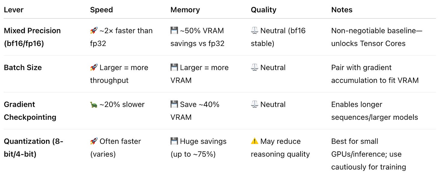
⚖️ Trade-Off Summary
These four techniques add to the foundation of efficient fine-tuning we covered in the previous post. This chart is a high-level overview of impact on our forces and priorities to give you a starting point, but its real impact can vary in application nuance.
🧪 Practical Workflow to Expand Your Setup
Now that you understand the trade-offs, here’s how to apply these levers in practice.
🧭 Strategy Mindset
Think of optimization as navigation, not force. Start with one stable configuration, then explore by changing a single parameter at a time. Track how it affects both quality and resource use. Build a personal map of what works best for your hardware and data rather than copying “optimal” configs blindly.
This approach helps prevent burnout and ensures each improvement is grounded in real measurement, not hype.
✅ Quick Wins
- Start bf16: true (or fp16: true fallback), micro_batch_size: 1, tune gradient_accumulation_steps, and turn on checkpointing if VRAM is tight.
- Increase GA until utilization is high and loss is smooth.
- Only then consider quantization: “8bit” or “4bit”; re‑check task quality.
❌ Common Pitfalls
- Confusing micro‑batch with effective batch (forgetting devices/GA).
- Enabling 4‑bit without a non‑quantized baseline.
- Assuming “flash attention” is on—verify in logs / profiler.
- VRAM fragmentation over long runs—periodically restart if creep appears.
📦 Starter Config Examples (Axolotl)
Baseline (quality-first; bf16‑capable GPUs like A100/H100)
yaml

# Precision
bf16: true            # quality-neutral vs fp32 on most tasks

# Memory helpers
gradient_checkpointing: true

# Throughput vs VRAM
micro_batch_size: 1
gradient_accumulation_steps: 8   # tune based on utilization

# Quantization
# (none)                  # keep unquantized for a true quality baseline
Constrained 24GB GPU (fit-first with QLoRA)
yaml

# Memory helpers
gradient_checkpointing: true
micro_batch_size: 1
gradient_accumulation_steps: 128   # long context or tight VRAM

# QLoRA quantization (4-bit NF4)
load_in_4bit: true
bnb_4bit_quant_type: nf4
bnb_4bit_use_double_quant: true
bnb_4bit_compute_dtype: bfloat16   # fallback to float16 if bf16 unsupported

# If 4-bit is unstable on your stack, try 8-bit instead:
# load_in_8bit: true
# (and remove the bnb_4bit_* keys)
💡 Key Insights
The techniques of batch size, mixed precision, quantization, and gradient checkpointing expand on your foundational optimization toolkit. Mixed precision is universal. Batch size and gradient accumulation let you balance throughput with VRAM constraints. Quantization becomes essential on consumer hardware. And gradient checkpointing? That’s often the difference between “it fits” and “it doesn’t.”
Master these levers in addition to the previous post, and you’ll have the fundamentals needed for stability in an llm fine-tuning project. The real skill isn’t knowing these techniques exist. It’s knowing which order to apply them and when to stop. Get to a stable mixed‑precision baseline, tune batch, add checkpointing if needed, then consider quantization based on hardware and quality requirements.
Finally, always ask the strategic question: is building your own model worth it? With foundation models improving rapidly, make sure the long-term value of your fine-tuned system outweighs the cost—especially if your product depends on owning it.
$ cd /posts/ — all posts